Gaussian Mixture Model 高斯混合模型 GMM

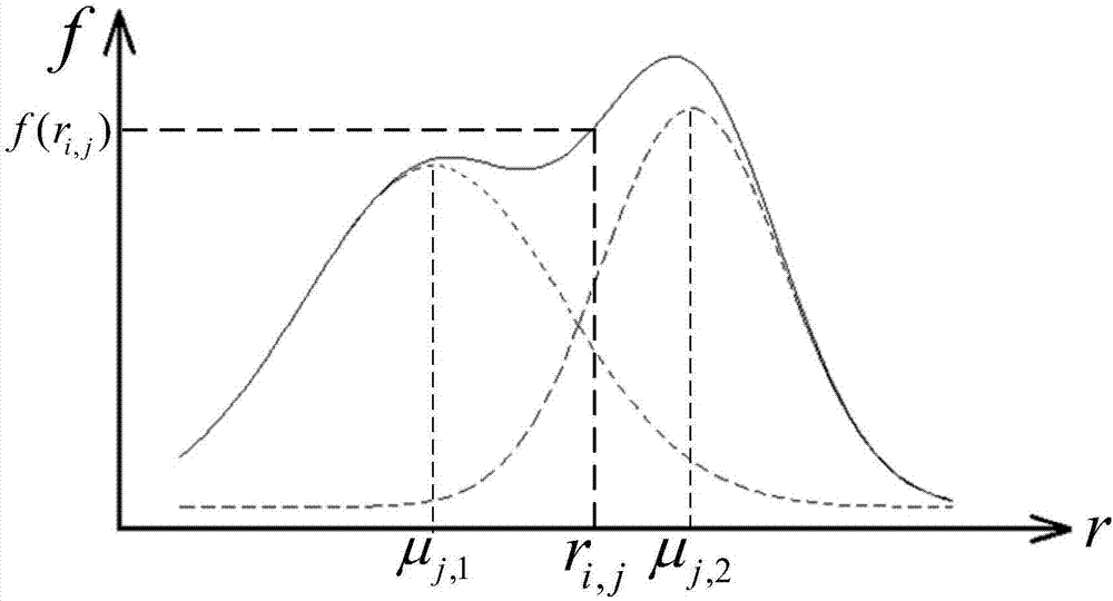
Gaussian Mixture Model 高斯混合模型 GMM

Gaussian mixture model is a combine of multiple Gaussian models. These Gaussian models mixture according to ‘weight’ $\pi$. The picture is a mixture of two models.

GMM

{ P ( X ∣ c ) = ∑ k = 1 K π k N ( x ( n ) ∣ μ k , Σ k ) N ( x ( n ) ∣ μ k , Σ k ) = 1 ( 2 π ) d 2 ∣ Σ k ∣ 1 2 e x p [ − 1 2 ( x ( n ) − μ k ) T Σ − 1 ( x ( n ) − μ k ) ] ∑ k = 1 K π k = 1 \left\{\begin{array}{l} P(X|c) = \sum\limits_{k=1}^K\pi_kN(x^{(n)}|\mu_k, \Sigma_k) \\ N(x^{(n)}|\mu_k, \Sigma_k) = \frac{1}{(2\pi)^{\frac d2}|\Sigma_k|^{\frac12}}exp[-\frac12(x^{(n)}-\mu_k)^T\Sigma^{-1}(x^{(n)}-\mu_k)] \\ \sum\limits_{k=1}^K \pi_k= 1 \end{array}\right. ⎩⎪⎪⎪⎪⎪⎨⎪⎪⎪⎪⎪⎧​P(X∣c)=k=1∑K​πk​N(x(n)∣μk​,Σk​)N(x(n)∣μk​,Σk​)=(2π)2d​∣Σk​∣21​1​exp[−21​(x(n)−μk​)TΣ−1(x(n)−μk​)]k=1∑K​πk​=1​

π k \pi_k πk​ – the probability of one example belongs to the k t h k^{th} kth Gaussian model/the weight of k t h k^{th} kth model in the mixture model

Attention! GMM is not a convex function and it has local optima(k local optima). What shall we do?
Strategies:
(i) gradient descent
(ii) heuristic algorithm including Simulated Annealing, Evolutionary Algorithms, etc (People hardly use these algorithms nowadays)
(iii)EM algorithm Today’s superstar

EM Algorithm for GMM

general EM Algorithm

Pros and cons

Cons:

1. EM algorithm is not a general algorithm dealing with non-convex problem.

Pros:

1. No hyper-parameters
2. Simple coding work
3. Theoretically graceful

EM for GMM

γ n k \gamma_{nk} γnk​ – the probability of x ( n ) x^{(n)} x(n) belongs to k t h k^{th} kth model
N k N_k Nk​ – the expectation of #examples belong to k t h k^{th} kth model

r a n d o m i z e { π k , μ k , Σ k } k = 1 ∼ K w h i l e ( ! c o n v e r g e ) { E − s t e p : γ n k = π k N ( x n ∣ μ k , Σ k ) ∑ k = 1 K N ( x n ∣ μ k , Σ k ) M − s t e p : N k = ∑ k = 1 K γ n k f o r ( k m o d e l s ) { π k ( n e w ) = N k N μ k ( n e w ) = 1 N k ∑ n = 1 N γ n k x ( n ) Σ k ( n e w ) = 1 N k ∑ n = 1 N γ n k [ x ( n ) − μ k ( n e w ) ] [ x ( n ) − μ k ( n e w ) ] T { } randomize \{\pi_k,\mu_k,\Sigma_k\}_{k=1\sim K} \\ while (!converge) \\ \{ \\ \ \ \ \ \ \ \ \ E-step: \ \\ \ \ \ \ \ \ \ \ \ \ \ \ \ \ \ \ \gamma_{nk} = \frac{\pi_kN(x_n|\mu_k, \Sigma_k)}{\sum\limits_{k=1}^KN(x_n|\mu_k, \Sigma_k)} \\ \ \ \ \ \ \ \ \ M-step: \ \\ \ \ \ \ \ \ \ \ \ \ \ \ \ \ \ \ N_k= \sum\limits_{k=1}^K\gamma_{nk} \\ \ \ \ \ \ \ \ \ \ \ \ \ \ \ \ \ for(k \ models) \\ \ \ \ \ \ \ \ \ \ \ \ \ \ \ \ \ \{ \\ \ \ \ \ \ \ \ \ \ \ \ \ \ \ \ \ \ \ \ \ \ \ \ \ \pi_k^{(new)}=\frac{N_k}{N} \\ \ \ \ \ \ \ \ \ \ \ \ \ \ \ \ \ \ \ \ \ \ \ \ \ \mu_k^{(new)} = \frac{1}{N_k}\sum\limits_{n=1}^N\gamma_{nk}x^{(n)} \\ \ \ \ \ \ \ \ \ \ \ \ \ \ \ \ \ \ \ \ \ \ \ \ \ \Sigma_k^{(new)} = \frac{1}{N_k}\sum\limits_{n=1}^N\gamma_{nk}[x^{(n)}-\mu_k^{(new)}] [x^{(n)}-\mu_k^{(new)}] ^T \\ \ \ \ \ \ \ \ \ \ \ \ \ \ \ \ \ \{ \\ \} randomize{πk​,μk​,Σk​}k=1∼K​while(!converge){        E−step:                 γnk​=k=1∑K​N(xn​∣μk​,Σk​)πk​N(xn​∣μk​,Σk​)​        M−step:                 Nk​=k=1∑K​γnk​                for(k models)                {                        πk(new)​=NNk​​                        μk(new)​=Nk​1​n=1∑N​γnk​x(n)                        Σk(new)​=Nk​1​n=1∑N​γnk​[x(n)−μk(new)​][x(n)−μk(new)​]T                {}
We use soft discrimination in this application of EM algorithm, which means we will compute the probability of each examples belongs to all models. In other applictions, take K-Means clustering algorithm for example, we use winner-takes-all strategy.