impedance用于阻抗谱拟合的Python库，bode图的优化方法，impedance输出bode图的优化方法

目录

1、优化原因

2、异常原因分析

3、修改方法

1、优化原因

下面是一段用impedance拟合一条阻抗数据的代码示例

from impedance.preprocessing import readGamry
from impedance.preprocessing import ignoreBelowX
from impedance.models.circuits import CustomCircuit
import matplotlib.pyplot as pltf, Z = readGamry('171018-1247_#54.DTA')     #读取数据
f, Z = ignoreBelowX(f, Z)                      #整理数据initial_guess = [2.29e-10, 0.98, 3.08E+5, 4.63E+5, 1.12E+6,1.57E-16,9.8E-5,5.07E+9]         #给定电路元器件初值
circuit = CustomCircuit('p(CPE_0,R_0)-p(C_0,W_0-R_1)-p(C_1,R_2)',initial_guess=initial_guess)     #给定等效电路结构 'p(CPE_0,R_0)-p(Q_0,W_0-R_1)-p(Q_1,R_2)'circuit.fit(f, Z)                  #拟合等效电路参数
print(circuit)                     #输出拟合结果circuit.plot(f_data=f, Z_data=Z, kind='bode')          #拟合结果可视化
plt.show()

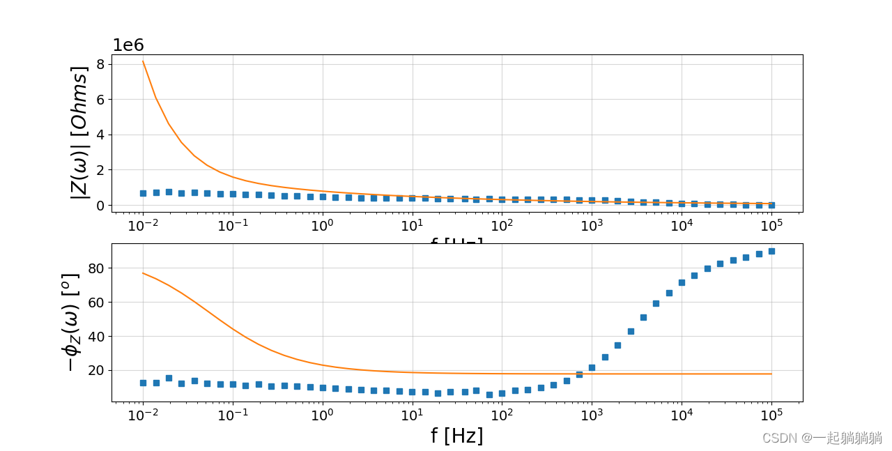
输出的bode图 

来对比一下普遍使用的阻抗谱bode图

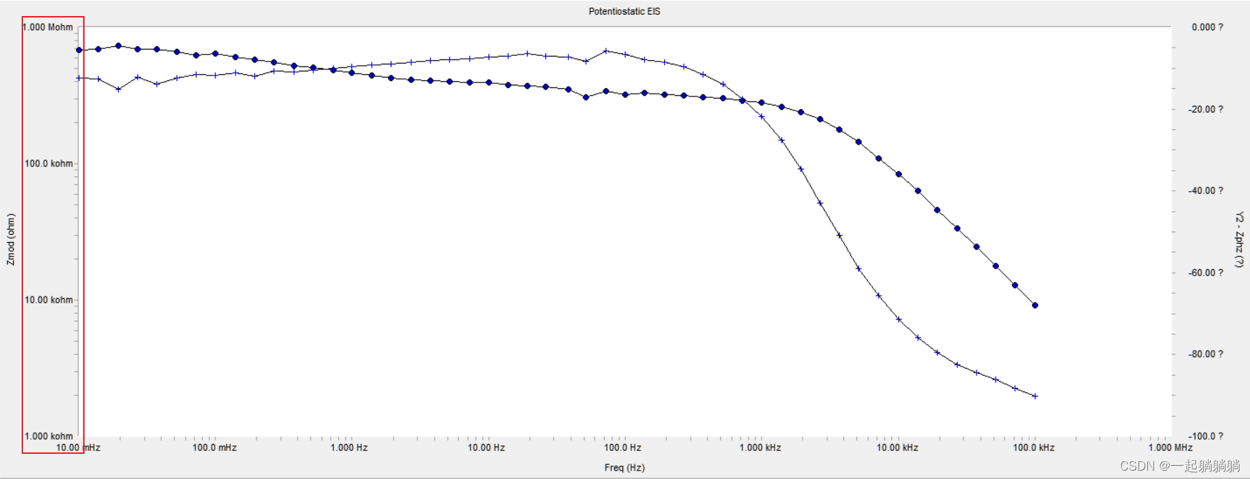
第一张图中的蓝色点是原始数据点，这两张图的数据是一样的，是不是看着这个图形差距很大，注意看图2中的红色框，纵坐标是对数轴，而图一纵坐标是以log为底的，显然坐标尺度不一样那图形可视化出来肯定不一样，

2、异常原因分析

为了改变这个图的坐标尺度，我看了circuit.plot这个函数的代码，代码如下，只需要改动bode图，我就只复制了其中bode图的代码

def plot(self, ax=None, f_data=None, Z_data=None, kind='altair', **kwargs):if kind == 'nyquist':#。。。。。略elif kind == 'bode':if ax is None:_, ax = plt.subplots(nrows=2, figsize=(5, 5))if f_data is not None:f_pred = f_dataelse:f_pred = np.logspace(5, -3)if Z_data is not None:if f_data is None:raise ValueError('f_data must be specified if' +' Z_data for a Bode plot')ax = plot_bode(f_data, Z_data, ls='', marker='s',axes=ax, **kwargs)if self._is_fit():Z_fit = self.predict(f_pred)ax = plot_bode(f_pred, Z_fit, ls='-', marker='',axes=ax, **kwargs)return ax

可以看到下面代码是画图的代码

ax = plot_bode(f_data, Z_data, ls='', marker='s',

                               axes=ax, **kwargs)

用到了plot_bode这个函数，在头文件中发现

from impedance.visualization import plot_altair, plot_bode, plot_nyquist

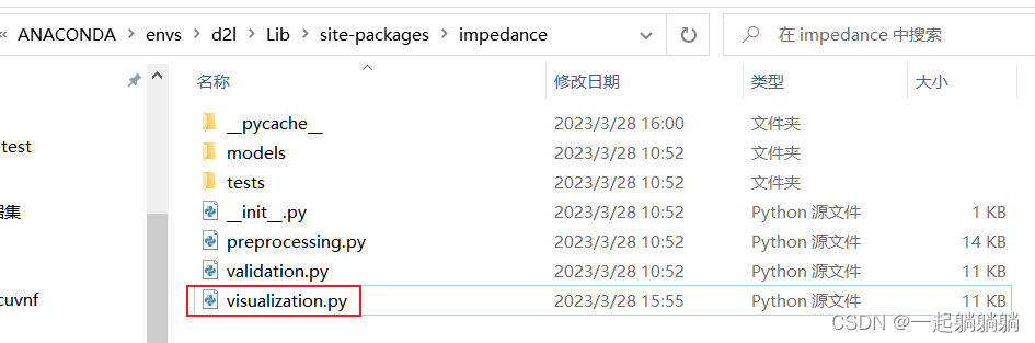
这个定义，下面就去找visualization.py这个文件，我图中显示出了这个文件的路径，可自行对应

打开该文件后，找到plot_bode

def plot_bode(axes, f, Z, scale=1, units='Ohms', fmt='.-', **kwargs):ax_mag, ax_phs = axesax_mag.plot(f, np.abs(Z), fmt, **kwargs)ax_phs.plot(f, -np.angle(Z, deg=True), fmt, **kwargs)# Set the y-axis labelsax_mag.set_ylabel(r'$|Z(\omega)|$ ' +'$[{}]$'.format(units), fontsize=20)ax_phs.set_ylabel(r'$-\phi_Z(\omega)$ ' + r'$[^o]$', fontsize=20)for ax in axes:# Set the frequency axes title and make log scaleax.set_xlabel('f [Hz]', fontsize=20)ax.set_xscale('log')# Make the tick labels largerax.tick_params(axis='both', which='major', labelsize=14)# Change the number of labels on each axis to fiveax.locator_params(axis='y', nbins=5, tight=True)# Add a light gridax.grid(b=True, which='major', axis='both', alpha=.5)# Change axis units to 10**log10(scale) and resize the offset textlimits = -np.log10(scale)if limits != 0:ax_mag.ticklabel_format(style='sci', axis='y',scilimits=(limits, limits))y_offset = ax_mag.yaxis.get_offset_text()y_offset.set_size(18)return axes

可以看到这个函数是用plot来画bode图的，x为对数轴是因为ax.set_xscale('log')设置了x为对数轴，该函数是把模值和相角分开画的，for ax in axes:这个循环统一设置了两个图形的格式和图标等，想知道里面具体格式设置信息的可以自行对应查找for中每个函数的意义。

x轴被设置为了对数轴，y轴只是最后设置了一下科学计数法表示，其还是按等距显示

3、修改方法

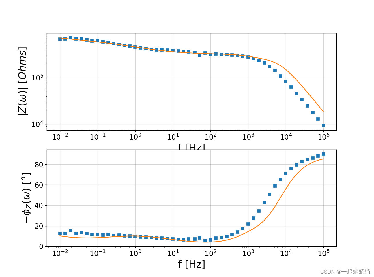
该函数也是用matplotlib来画图的，在matplotlib中可以用loglog来画双对数轴的图，semilogx可以画X为对数轴的图形，将两个plot改成用loglog画模值图，semilogx画相角图，并且把循环中的set_xscale、ax.locator_params注释掉

def plot_bode(f, Z, scale=1, units='Ohms', fmt='.-', axes=None, labelsize=20,ticksize=14, **kwargs):Z = np.array(Z, dtype=complex)if axes is None:_, axes = plt.subplots(nrows=2)ax_mag, ax_phs = axes#old'''ax_mag.plot(f, np.abs(Z), fmt, **kwargs)                  ax_phs.plot(f, -np.angle(Z, deg=True), fmt, **kwargs)'''#新的ax_mag.loglog(f, np.abs(Z), fmt, **kwargs)                ax_phs.semilogx(f, -np.angle(Z, deg=True), fmt, **kwargs)# Set the y-axis labelsax_mag.set_ylabel(r'$|Z(\omega)|$ ' +'$[{}]$'.format(units), fontsize=labelsize)ax_phs.set_ylabel(r'$-\phi_Z(\omega)$ ' + r'$[^o]$', fontsize=labelsize)for ax in axes:# Set the frequency axes title and make log scaleax.set_xlabel('f [Hz]', fontsize=labelsize)#注释掉了#ax.set_xscale('log')# Make the tick labels largerax.tick_params(axis='both', which='major', labelsize=ticksize)# Change the number of labels on each axis to five#注释掉了#ax.locator_params(axis='y', nbins=5, tight=True)   # Add a light gridax.grid(visible=True, which='major', axis='both', alpha=.5)# Change axis units to 10**log10(scale) and resize the offset textlimits = -np.log10(scale)if limits != 0:ax_mag.ticklabel_format(style='sci', axis='y',scilimits=(limits, limits))y_offset = ax_mag.yaxis.get_offset_text()y_offset.set_size(18)return axes

再次运行输出图形如下 

 这个需要修改的py文件路径可以再图三看到，我的路径如下D:\work apps\ENVS\ANACONDA\envs\d2l\Lib\site-packages\impedance