
基于上次的文章再次进行补充:http://t.csdn.cn/75EPC
在这篇文章开始前,我使用了模型《Relation-Aware Global Attention》去进行实践,但是环境配置一直出现问题,首先是环境配置的问题,torch与numpy的版本无法正常的匹配,还要无法检测到torch的一些函数等等问题,这一篇主要是要针对《Relation Network for Person Re-identification》这篇论文进行实践。
目录
0x01 基于行人局部特征融合的再识别实战
(一)数据集的准备
(二)参数配置
(三)配置环境依赖
(四)数据源构建方法分析
(五)dataloader加载顺序解读
(六)网络计算整体流程
(七)损失函数
(八)开始训练以及测试
0x01 基于行人局部特征融合的再识别实战
(一)数据集的准备
pid(人)+摄像头的编号+每个摄像头对应的图片id:
 那么数据集的文件下就有这些文件:
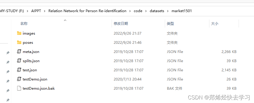
可以注意到有一个名称为poses的文件,这个文件是用于训练检测人体姿态的信息,用于姿态估计,在这个当前的情景下我们是用不上了,可以删掉。
再看看json文件:
splits.json是数据集的划分。
meta.json是数据集的对每个人每组摄像头的数据进行处理,将每个人的数据以及对应的摄像头为一组,使用【】括起来,最后再把每个人的数据全都括起来:

(二)参数配置
使用pycharm打开下载好的源码,之后可以发现有这么几行参数:
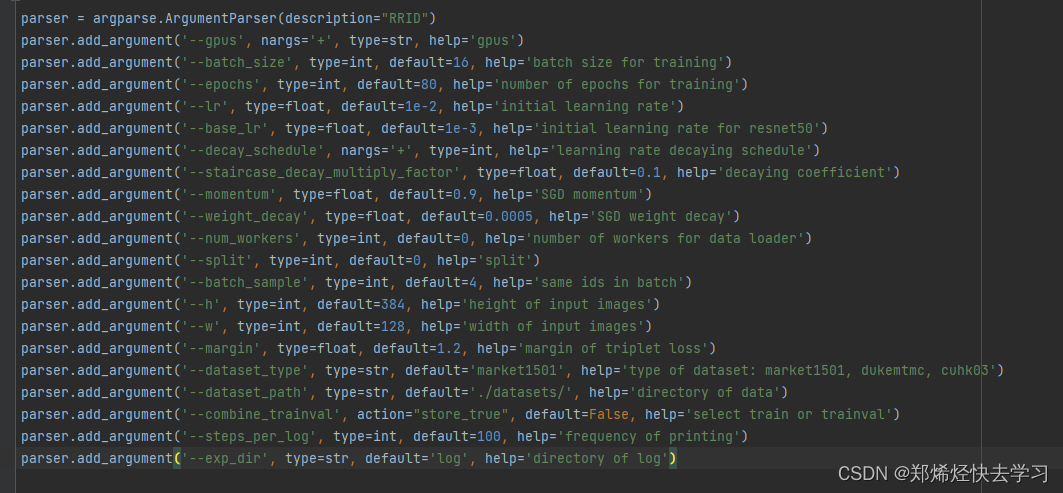
在训练的时候指定GPU就可以了,比如我刚开始训练在py文件后带上:--gpus 0。源码GitHub在这里:https://github.com/cvlab-yonsei/RRID
(三)配置环境依赖
Python 3.6
PyTorch >= 0.4.1
numpy
h5py
那么就使用anaconda来进行配置叭:
conda create -n RRID python==3.6
conda activate RRID
这里我是使用gpu跑的,安装符合要求的pytorch:
conda install pytorch==1.8.0 torchvision==0.9.0 torchaudio==0.8.0 cudatoolkit=10.2 -c pytorch
conda install numpy
conda install h5py
(四)数据源构建方法分析
构建dataset:
# Dataset Loader
dataset, train_loader, val_loader, _ = get_data(args.dataset_type, args.split, args.dataset_path, args.h, args.w, args.batch_size, args.num_workers, args.combine_trainval, np_ratio)
在train.py文件中有这么一句处理数据的函数,可以进入get_data函数中看看:
def get_data(name, split_id, data_dir, height, width, batch_size, workers,combine_trainval, np_ratio):#数据集路径root = osp.join(data_dir, name)dataset = datasets.create(name, root, split_id=split_id)#normalizer = T.Normalize(mean=[0.485, 0.456, 0.406],std=[0.229, 0.224, 0.225])train_set = dataset.trainval if combine_trainval else dataset.traintrain_transformer = T.Compose([T.RectScale(height, width),T.RandomSizedEarser(),T.RandomHorizontalFlip(),T.ToTensor(),normalizer,])test_transformer = T.Compose([T.RectScale(height, width),T.ToTensor(),normalizer,])#train_loader = DataLoader(Preprocessor(train_set, root=dataset.images_dir,transform=train_transformer),sampler=TripletBatchSampler(train_set),batch_size=batch_size, num_workers=workers, pin_memory=False)val_loader = DataLoader(Preprocessor(dataset.val, root=dataset.images_dir,transform=test_transformer),batch_size=batch_size, num_workers=workers,shuffle=False, pin_memory=False)test_loader = DataLoader(Preprocessor(list(set(dataset.query) | set(dataset.gallery)),root=dataset.images_dir, transform=test_transformer),batch_size=batch_size, num_workers=workers,shuffle=False, pin_memory=False)return dataset, train_loader, val_loader, test_loader那么我们先研究这个Preprocessor的这个类吧,然后关注一下构建数据的这个函数:

之后再回去关注一下sampler这个变量,在以往的神经网络中,这个时候是要对数据集进行随机提取,但是在这里要进行三元组损失的提取,所以不可以进行随机提取,需要自己写函数进行处理:
class TripletBatchSampler(Sampler):def __init__(self, data_source, batch_image=4):super(TripletBatchSampler, self).__init__(data_source)self.data_source = data_sourceself.num_samples = len(data_source)self.batch_image = batch_image# Sort by pidindices = np.argsort(np.asarray(data_source)[:, 1])self.index_map = dict(zip(np.arange(self.num_samples), indices))# Get the range of indices for each pidself.index_range = defaultdict(lambda: [self.num_samples, -1])for i, j in enumerate(indices):_, pid, _ = data_source[j]self.index_range[pid][0] = min(self.index_range[pid][0], i)self.index_range[pid][1] = max(self.index_range[pid][1], i)#迭代时如何拿到索引def __iter__(self):indices = np.random.permutation(self.num_samples)for i in indices:# anchor sampleanchor_index = self.index_map[i]_, pid, _ = self.data_source[anchor_index]# positive samplestart, end = self.index_range[pid]pos_indices = _choose_from(start, end, excluded_range=(i, i), size=self.batch_image)for pos_index in pos_indices:yield self.index_map[pos_index]def __len__(self):return self.num_samples*self.batch_image所以上面这个类的作用是不断返回实际的索引,这个采样的操作是先处理的。
(五)dataloader加载顺序解读
在dataset.py中读取各种json文件:
def load(self, num_val=0.3, verbose=True):splits = read_json(osp.join(self.root, 'testDemo.json'))#splits = read_json(osp.join(self.root, 'splits.json'))if self.split_id >= len(splits):raise ValueError("split_id exceeds total splits {}".format(len(splits)))self.split = splits[self.split_id]trainval_pids = sorted(np.asarray(self.split['trainval']))num = len(trainval_pids)if isinstance(num_val, float):num_val = int(round(num * num_val))if num_val >= num or num_val < 0:raise ValueError("num_val exceeds total identities {}".format(num))train_pids = sorted(trainval_pids[:-num_val])val_pids = sorted(trainval_pids[-num_val:])self.meta = read_json(osp.join(self.root, 'meta.json'))identities = self.meta['identities']self.train, self.train_query = _pluck(identities, train_pids, relabel=True)self.val, self.val_query = _pluck(identities, val_pids, relabel=True)self.trainval, self.trainval_query = _pluck(identities, trainval_pids, relabel=True)self.test_list = read_json(osp.join(self.root, 'test.json'))[0]for i in range(len(self.test_list['query'])):self.test_list['query'][i] = tuple(self.test_list['query'][i])for i in range(len(self.test_list['gallery'])):self.test_list['gallery'][i] = tuple(self.test_list['gallery'][i])self.query = self.test_list['query']self.gallery = self.test_list['gallery']self.num_train_ids = len(train_pids)self.num_val_ids = len(val_pids)self.num_trainval_ids = len(trainval_pids)if verbose:print(self.__class__.__name__, "dataset loaded")print(" subset | # ids | # images")print(" ---------------------------")print(" train | {:5d} | {:8d}".format(self.num_train_ids, len(self.train)))print(" val | {:5d} | {:8d}".format(self.num_val_ids, len(self.val)))print(" trainval | {:5d} | {:8d}".format(self.num_trainval_ids, len(self.trainval)))print(" query | {:5d} | {:8d}".format(len(self.split['query']), len(self.query)))print(" gallery | {:5d} | {:8d}".format(len(self.split['gallery']), len(self.gallery)))其中的pluck函数就是读取数据集的操作了:
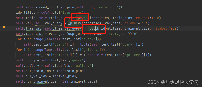
def _pluck(identities, indices, relabel=False):ret = []query = {}for index, pid in enumerate(indices):pid_images = identities[pid] # 得到当前pid的所有数据if relabel:if index not in query.keys():query[index] = []else:if pid not in query.keys():query[pid] = []for camid, cam_images in enumerate(pid_images):for fname in cam_images:name = osp.splitext(fname)[0]x, y, _ = map(int, name.split('_'))
#                 assert pid == x and camid == yif relabel:ret.append((fname, index, camid))# 图像 人编号 相机编号query[index].append(fname)else:ret.append((fname, pid, camid))query[pid].append(fname)return ret, query
上面这个函数就可以通过我们的标题来获取我们图像的数据信息了。
之后获取到图像数据信息后,可以通过sampler.py下的一个函数来进行随机读取:
def __iter__(self):indices = np.random.permutation(self.num_samples)for i in indices:# anchor sampleanchor_index = self.index_map[i]_, pid, _ = self.data_source[anchor_index]# positive samplestart, end = self.index_range[pid]pos_indices = _choose_from(start, end, excluded_range=(i, i), size=self.batch_image)for pos_index in pos_indices:yield self.index_map[pos_index]在这个函数中在人物数据中选取几张进行下一步,之后进行返回,要返回所有batch_size的索引。
接下来是要读取索引的图像,在preprocesssor.py中,对索引进行读取,首先要判断是否读取人体姿态:
def __getitem__(self, indices):if isinstance(indices, (tuple, list)):if not self.with_pose:return [self._get_single_item(index) for index in indices]else:return [self._get_single_item_with_pose(index) for index in indices]if not self.with_pose:return self._get_single_item(indices)else:return self._get_single_item_with_pose(indices)def _get_single_item(self, index):fname, pid, camid = self.dataset[index]fpath = fnameif self.root is not None:fpath = osp.join(self.root, fname)img = Image.open(fpath).convert('RGB')img = self.transform(img)return img, fname, pid, camid第一个函数是选择模式,是否需要读取人体姿态,下面的则是对图像信息进行提取,之后进行transform,transform的参数已经在上面配置好了:
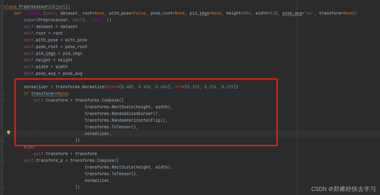
做了预处理+数据增强。
那么上面就是对数据的处理了,处理完之后则需要构建网络模型:

基于resnet50网络结构:

其中的resnet50在我们文件夹中已经有现成的了,调用就行。

(六)网络计算整体流程
def forward(self, x):criterion = nn.CrossEntropyLoss()#print(x.shape) # 8 3 384 128 feat = self.base(x) # 8 3 2048 24 8#print(feat.shape) assert (feat.size(2) % self.num_stripes == 0)stripe_h_6 = int(feat.size(2) / self.num_stripes) # 4stripe_h_4 = int(feat.size(2) / 4) # 6stripe_h_2 = int(feat.size(2) / 2) # 12local_6_feat_list = []local_4_feat_list = []local_2_feat_list = []final_feat_list = []logits_list = []rest_6_feat_list = []rest_4_feat_list = []rest_2_feat_list = []logits_local_rest_list = []logits_local_list = []logits_rest_list = []logits_global_list = []类似于stripe_h_6这样的操作,其实就是把图像进行分割成几份进行提取特征。之后local分别用于存储他们的特征。
各种初始化做完后,就对图像进行提取特征:
for i in range(self.num_stripes): # 得到6块中每一个的特征local_6_feat = F.max_pool2d(feat[:, :, i * stripe_h_6: (i + 1) * stripe_h_6, :], # 每一块是4*w(stripe_h_6, feat.size(-1))) #pool成1*1的#print(local_6_feat.shape) #8 2048 1 1local_6_feat_list.append(local_6_feat) # 按顺序得到每一块的特征下面是进行GCP全局特征提取模块:
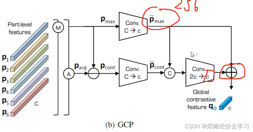
global_6_max_feat = F.max_pool2d(feat, (feat.size(2), feat.size(3))) # 8 2048 1 1,全局特征#print(global_6_max_feat.shape)global_6_rest_feat = (local_6_feat_list[0] + local_6_feat_list[1] + local_6_feat_list[2]#局部与全局的差异 + local_6_feat_list[3] + local_6_feat_list[4] + local_6_feat_list[5] - global_6_max_feat)/5#print(global_6_rest_feat.shape) # 8 2048 1 1global_6_max_feat = self.global_6_max_conv_list[0](global_6_max_feat) # 8 256 1 1#print(global_6_max_feat.shape)global_6_rest_feat = self.global_6_rest_conv_list[0](global_6_rest_feat) # 8 256 1 1#print(global_6_rest_feat.shape)global_6_max_rest_feat = self.global_6_pooling_conv_list[0](torch.cat((global_6_max_feat, global_6_rest_feat), 1))#print(global_6_max_rest_feat.shape) # 8 256 1 1global_6_feat = (global_6_max_feat + global_6_max_rest_feat).squeeze(3).squeeze(2)#print(global_6_feat.shape) # 论文中Global contrastive feature Figure2(b),得到256个特征先通过maxpool得到单独特征,之后将所有局部特征加在一起,再减去一个整体的特征操作,之后再求平均。其实就是这个过程:
下面是局部特征提取模块:
for i in range(self.num_stripes): #对于每块特征,除去自己之后其他的特征组合在一起rest_6_feat_list.append((local_6_feat_list[(i+1)%self.num_stripes]#论文公式1处的ri + local_6_feat_list[(i+2)%self.num_stripes]+ local_6_feat_list[(i+3)%self.num_stripes] + local_6_feat_list[(i+4)%self.num_stripes]+ local_6_feat_list[(i+5)%self.num_stripes])/5)for i in range(4):local_4_feat = F.max_pool2d(feat[:, :, i * stripe_h_4: (i + 1) * stripe_h_4, :],(stripe_h_4, feat.size(-1)))#print(local_4_feat.shape)local_4_feat_list.append(local_4_feat)上面其实就是对六个或者四个或者两个进行自己与其他人的关系,算法都是一样的。
之后进行一个pi操作:
for i in range(self.num_stripes):local_6_feat = self.local_6_conv_list[i](local_6_feat_list[i]).squeeze(3).squeeze(2)#pi#print(local_6_feat.shape)input_rest_6_feat = self.rest_6_conv_list[i](rest_6_feat_list[i]).squeeze(3).squeeze(2)#ri#print(input_rest_6_feat.shape)input_local_rest_6_feat = torch.cat((local_6_feat, input_rest_6_feat), 1).unsqueeze(2).unsqueeze(3)#print(input_local_rest_6_feat.shape) # 8 512 1 1local_rest_6_feat = self.relation_6_conv_list[i](input_local_rest_6_feat)#print(local_rest_6_feat.shape) # 8 256 1 1local_rest_6_feat = (local_rest_6_feat + local_6_feat.unsqueeze(2).unsqueeze(3)).squeeze(3).squeeze(2)#print(local_rest_6_feat.shape)# 16 256final_feat_list.append(local_rest_6_feat)其中进行了特征的拼接操作,再进行卷积,再进行加法操作。最后得到的结果进行存起来。
if self.num_classes > 0:logits_local_rest_list.append(self.fc_local_rest_6_list[i](local_rest_6_feat)) #当前local和rest的分类结果logits_local_list.append(self.fc_local_6_list[i](local_6_feat))# 当前local的分类结果logits_rest_list.append(self.fc_rest_6_list[i](input_rest_6_feat))# 当前rest的分类结果#print(np.array(logits_local_rest_list).shape)上面是one vs rest的部分,完成了分为六部分的计算,对应的是one vs rest的那个图。
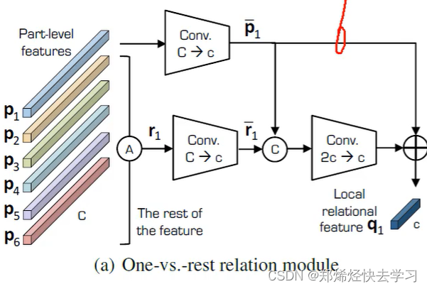
接下来是要得到所有分组特征结果: 由于我们分了六分、四份以及两份,所以最后一共有十二个预测结果。
if self.num_classes > 0:logits_local_rest_list.append(self.fc_local_rest_2_list[i](local_rest_2_feat))logits_local_list.append(self.fc_local_2_list[i](local_2_feat))logits_rest_list.append(self.fc_rest_2_list[i](input_rest_2_feat))   final_feat_list.append(global_6_feat)
final_feat_list.append(global_4_feat)
final_feat_list.append(global_2_feat)
#print(np.array(logits_local_rest_list).shape)
之后进行pi,对十二个预测结果进行分类,一共有九个分类任务:
if self.num_classes > 0:logits_global_list.append(self.fc_global_6_list[0](global_6_feat))logits_global_list.append(self.fc_global_max_6_list[0](global_6_max_feat.squeeze(3).squeeze(2)))logits_global_list.append(self.fc_global_rest_6_list[0](global_6_rest_feat.squeeze(3).squeeze(2)))logits_global_list.append(self.fc_global_4_list[0](global_4_feat))logits_global_list.append(self.fc_global_max_4_list[0](global_4_max_feat.squeeze(3).squeeze(2)))logits_global_list.append(self.fc_global_rest_4_list[0](global_4_rest_feat.squeeze(3).squeeze(2)))logits_global_list.append(self.fc_global_2_list[0](global_2_feat))logits_global_list.append(self.fc_global_max_2_list[0](global_2_max_feat.squeeze(3).squeeze(2)))logits_global_list.append(self.fc_global_rest_2_list[0](global_2_rest_feat.squeeze(3).squeeze(2)))#print(np.array(logits_global_list).shape)return final_feat_list, logits_local_rest_list, logits_local_list, logits_rest_list, logits_global_list以上就可以得到分类损失啦。也是我们前向传播的东西。
(七)损失函数
前向传播后会存储到这个地方:
final_feat_list, logits_local_rest_list, logits_local_list, logits_rest_list, logits_global_list = model(inputs)
前三个变量得到的是左边图的结果,最后一个变量得到的是右图的结果。
接下来是计算三元组损失:
T_loss = torch.sum(torch.stack([triplet_loss(output, labels) for output in final_feat_list]), dim=0)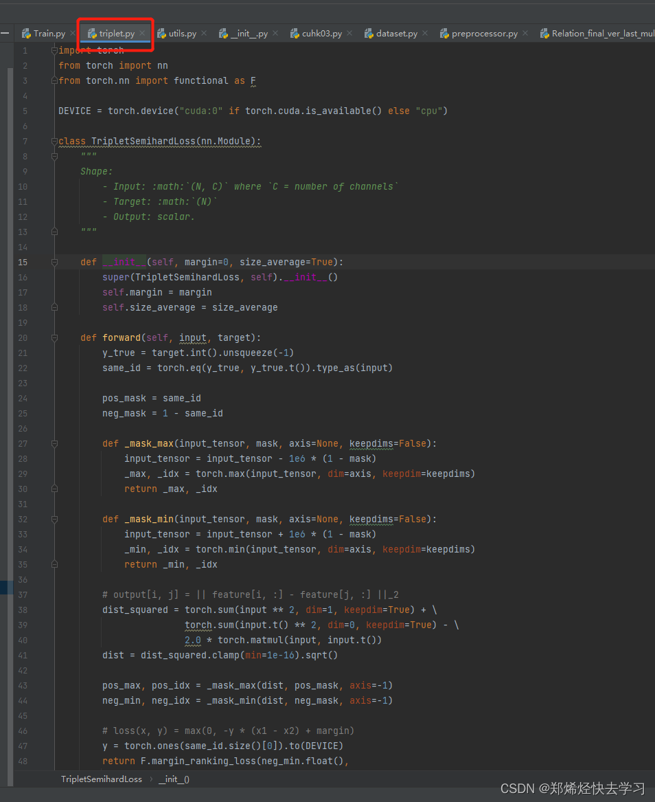
首先先获取样本的标签,构建矩阵,之后求其mask值,在同类中取最大以及不同类的最小值,然后进入距离计算公式:
dist_squared = torch.sum(input ** 2, dim=1, keepdim=True) + \torch.sum(input.t() ** 2, dim=0, keepdim=True) - \2.0 * torch.matmul(input, input.t())dist = dist_squared.clamp(min=1e-16).sqrt()pos_max, pos_idx = _mask_max(dist, pos_mask, axis=-1)neg_min, neg_idx = _mask_min(dist, neg_mask, axis=-1)# loss(x, y) = max(0, -y * (x1 - x2) + margin)y = torch.ones(same_id.size()[0]).to(DEVICE)之后将其return:
return F.margin_ranking_loss(neg_min.float(),pos_max.float(),y,self.margin,self.size_average)之后再使用交叉熵计算剩余的损失:
C_loss_local = torch.sum(torch.stack([cross_entropy_loss(output, labels) for output in logits_local_list]), dim=0)C_loss_local_rest = torch.sum(torch.stack([cross_entropy_loss(output, labels) for output in logits_local_rest_list]), dim=0)C_loss_rest = torch.sum(torch.stack([cross_entropy_loss(output, labels) for output in logits_rest_list]), dim=0)C_loss_global = torch.sum(torch.stack([cross_entropy_loss(output, labels) for output in logits_global_list]), dim=0)C_loss = C_loss_local_rest + C_loss_global + C_loss_local + C_loss_restloss = T_loss + 2 * C_losslosses.update(loss.data.item(), labels.size(0))再使用梯度下降进行参数更新,不断随着epoch进行迭代更新。
(八)开始训练以及测试
-
在目录下运行Train.py,附上“--gpus 0”,速度会比较慢,大概需要好几个小时。
-
测试需要输入:
--gpus 0
--pretrained_weights_dir pretrained_weights.pth
测试主要是在Evaluate.py文件中,在Evaluate.py后面赋予上面两个参数即可。
这个是其他参数:
parser = argparse.ArgumentParser(description="RRID")
parser.add_argument('--gpus', nargs='+', type=str, help='gpus')
parser.add_argument('--batch_size', type=int, default=16, help='mini-batch size for training')
parser.add_argument('--num_workers', type=int, default=0, help='number of workers for data loader')
parser.add_argument('--split', type=int, default=0, help='split')
parser.add_argument('--batch_sample', type=int, default=4, help='same ids in batch')
parser.add_argument('--h', type=int, default=384, help='height of input images')
parser.add_argument('--w', type=int, default=128, help='width of input images')
parser.add_argument('--dataset_type', type=str, default='market1501', help='type of dataset: market1501, dukemtmc, cuhk03')
parser.add_argument('--dataset_path', type=str, default='./datasets/', help='directory of data')
parser.add_argument('--print_freq', type=int, default=10, help='frequency of printing')
parser.add_argument('--exp_dir', type=str, default='log', help='directory of log')
parser.add_argument('--combine_trainval', action="store_true", default=False, help='select train or trainval')
parser.add_argument('--pretrained_weights_dir', type=str, default=None, help='pretrained weights')
这个是在测试过程中得到的参数:
with torch.no_grad():for i, (imgs, fnames, pids, _) in enumerate(test_loader):data_time.update(time.time() - end)imgs_flip = torch.flip(imgs, [3])final_feat_list, _, _, _, _, = model(Variable(imgs).cuda())final_feat_list_flip, _, _, _, _ = model(Variable(imgs_flip).cuda())for j in range(len(final_feat_list)):if j == 0:outputs = (final_feat_list[j].cpu() + final_feat_list_flip[j].cpu())/2else:outputs = torch.cat((outputs, (final_feat_list[j].cpu() + final_feat_list_flip[j].cpu())/2), 1)outputs = F.normalize(outputs, p=2, dim=1)for fname, output, pid in zip(fnames, outputs, pids):features[fname] = outputlabels[fname] = pidbatch_time.update(time.time() - end)end = time.time()if (i + 1) % args.print_freq == 0:print('Extract Features: [{}/{}]\t''Time {:.3f} ({:.3f})\t''Data {:.3f} ({:.3f})\t'.format(i + 1, len(test_loader),batch_time.val, batch_time.avg,data_time.val, data_time.avg))即可拿到每张图像的特征,给出实际特征、label、以及对应的pid。之后进行相似度的计算:
#Evaluating distance matrix
distmat = evaluators.pairwise_distance(features, dataset.query, dataset.gallery)